Using the SWITCHES database

This example does the following:

1. Downloads a bistable model from the SWITCHES database.
2. Describes how a model is written in SWITCHES format.
3. Describes how bistable parameters are extracted for the database using Latin Hypercube Sampling and by finding steady-states using MOOSE.
4. Demonstrates deterministic and stochastic time-course simulation in MOOSE to visualize bistability.

import warnings
warnings.filterwarnings("ignore")
warnings.simplefilter("ignore")

import requests
import moose
import matplotlib
%matplotlib notebook
import matplotlib.pyplot as plt
from mpl_toolkits.mplot3d import Axes3D
from string import ascii_lowercase as al
import numpy as np
import lhsmdu

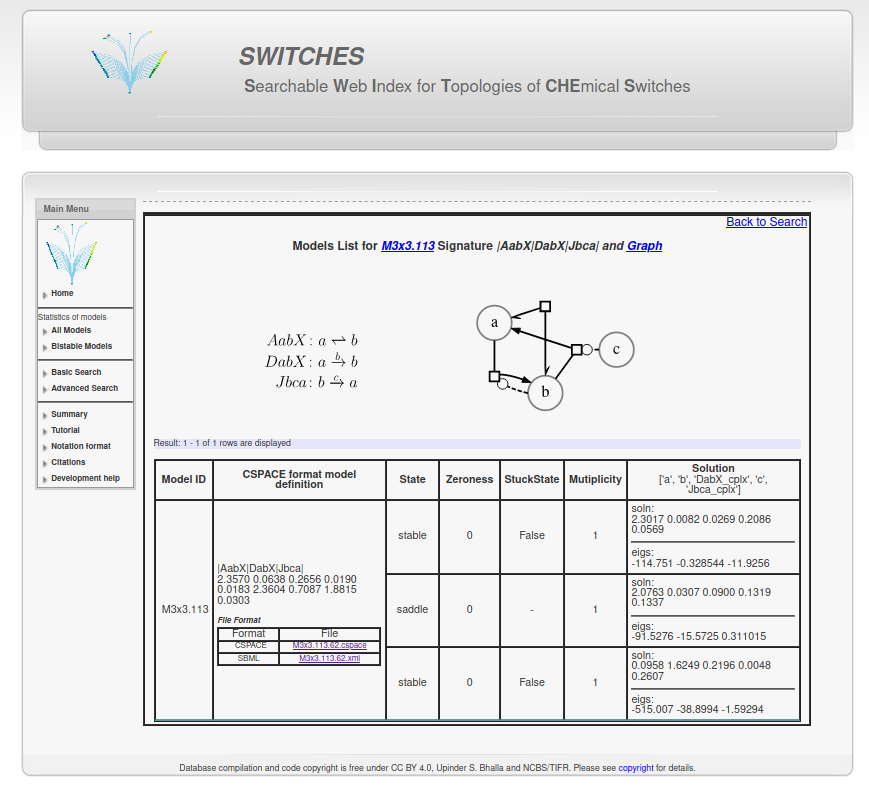
1. Downloading a CSPACE file from the SWITCHES database

1.1 Click on the "Bistable Models" in the left menu bar from the website homepage at http://switches.ncbs.res.in.

1.2 Select a model configuration size. In this example, we select 3x3 i.e. 3 reactions between 3 reactants.

1.3 Select a Model ID from this list. Here we pick M3x3.113.

1.4 You can also search by configuration size or other parameters using the basic and advanced search functionality on the left menu bar.

1.5 Save the CSPACE (or SBML) file for further use.

This page displays the model structure on top with selected bistable model parameters and solutions. On top, you can see the chemical reaction on the left with corresponding chemical reaction network in the SBGN format on the right.

1.6 Alternatively, get the CSPACE file directly from Python

url = 'https://switches.ncbs.res.in/file/M3x3.113.62.cspace'
r = requests.get(url, allow_redirects=True)
open('M3x3.113.62.cspace', 'wb').write(r.content)

---

modelName = "M3x3.113.62.cspace"

2. SWITCHES format

def parseTopology(model):
    readModel = open(model,'r')
    modelData = readModel.readlines()
    elements = modelData[0].split(' ')
    modelName, modelString, reactionPars = elements[0][:-1], elements[1], elements[2:]
    return modelName, modelString, reactionPars

def findNumReacs(modelString, reactionPars):
    ''' Finds the number of molecules and reactions in the topology '''
    reactionList = modelString.split('|')
    reactionDim = len(reactionList)-2 ## To get rid of the first and the last empty list and each reaction has 2 rates
    return reactionDim

2.1 SWITCHES format is a compact representation of a chemical reaction network.

It has three parts, model ID, model string, and the reaction parameters.

modelID, modelString, reactionPars = parseTopology(modelName)

print(modelID)

M3x3.113.62

2.2 Model ID is a hierarchical description of the model.

Level 1: M3x3 : Describes that the model has 3 reactants and 3 reactions respectively.

Level 2: 113 : Uniquely identifies the model string or the reaction network without the parameters.

Level 3: 62 : Uniquely identifies the reaction parameters of this reaction network.

print(modelString)

|AabX|DabX|Jbca|

2.3 Model string describes all the reactant and reactions in the reaction network.